RNA
Repository for RNA.
RNA (Rhythm-Note Alignment)
This is the description page for RNA, a symbolic music similarity measure using a modified version of local alignment. RNA uses a substitution function which consider the pitch class and the difference in the onset for each possible match. We also present a comparison made with these other similarity measures:
- Euclidean Distance
- Correlation Distance
- City Block Distance
- Local Alignment
- SIAM
- BSpline
Based on the work by Janssen, et. al. (2015) and Janssen, et. al. (2017). We use the same MTC-ANN dataset, version 2.0.1, available here, the pieces were preprocessed just to change the extension to musicxml files.
The following sections describe the experiments and link to the code used on each one.
- How it works?
- Controlled Experiments
- Comparison with Expert annotations
- Case study using Impro-Visor
How it works?
Introduction
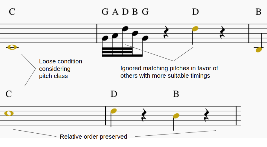
RNA comes from the intuiton that simple features such as pitch and duration can be of great use in analysis tasks like music similarity evaluations. It was first proposed to use the difference of start times of the notes as it is one of the most overlooked features on early similarity and distance measures tested. Also the penalizations for not matching strictly on the same pitch was worth of questioning if a more loose condition could improve the results. For this purpose the pitch matching is done using only the pitch class regardless on the octave. Now, just considering the amount of shared atomic elements like the ones described lack the judging of the more abstract structures present in music like the order in the melody, chords, motifs, etc. To tackle this issue an existing sequence matching algorithm was considered to modify and include the evaluation of the features described previously. The algorithm with the appropiate customization options that was selected is Local Alignment by considering its capabilites to consider relative order in the search of the longest common.
To give a final score we can define it as the relation between the length of the Longest Common Subsequence (LCS) and the length of the longest melody from the two compared melodies A and B. To this effect, the RNA between melodies A and B is calculated as follows:
\[RNA(\mathbf{A},\mathbf{B}) = 1 - \frac{|LCS_{\mathbf{A},\mathbf{B}}|}{\max{(|\mathbf{A}|,|\mathbf{B}|)}}\]To calculate the LCS between both melodies, we first need to eliminate their octave dependence, that is to say, notes are extracted regardless of the octave or the MIDI height in which they are located. Meaning, this representation takes all C notes as being of the same class, even though a C in the 3rd octave is lower than a C in the 5th octave. This is because, usually, only the relative distance with respect to the scale is taken into account when constructing chords and progression, and not their absolute distance in semitones.
Given two melodies A and B represented as a note class sequence, the LCS of notes can be calculated using the following recursive function:
\[\begin{split} &LCS(i,j) = \\ &\begin{cases} 0, \text{if } (i=0) \text{ or } (j=0) \\ \max{(LCS(i - 1,j), LCS(i,j - 1), LCS(i - 1,j - 1) + subs(i, j))}, \\ ~~~~~~\text{otherwise} \\ \end{cases} \end{split}\]where subs, is defined as:
\[\begin{split} &subs(i,j) = \\ &\begin{cases} 1, \\ ~~~~~~\text{if } (\mathbf{A}[i] = \mathbf{B}[j]) \text{ and }\\ ~~~~~~~~~~(\mathbf{P}_{A}[i] - \mathbf{P}_{B}[j]) < (\mathbf{P}_{A}[i] + \mathbf{P}_{B}[j]) / C_E\\ 0, otherwise \\ \end{cases} \end{split}\]where PA and PB are vectors calculated as:
\[\begin{split} \mathbf{P}_{A}[i] = start(\mathbf{A}[i]) - start(\mathbf{A}[i-1]) \\ \mathbf{P}_{B}[j] = start(\mathbf{B}[j]) - start(\mathbf{B}[j-1]) \end{split}\]where start returns the starting point of a given note; and, CE is a scaling coefficient, the value of which was experimentally obtained as half the average of a typical P vector; in this case, it has a value of 64. This was implemented in order to incorporate a threshold that could make the distiction of significant differences between the notes. In this case we calculate how much the difference should be in order to be noticeable for the algorithm. It wouldn’t be appropiate to define a fixed value because of how much different musical pieces could be, instead what is fixed is the scale related to the onset times of each song, with the hypothesis to being able to suit multiple melodic sets.
The cardinality of the LCSA,B factor in is inherently maximized when the LCS recursive function reaches a stop scenario (required similarly in the Local Alignment measure). To ensure this, the original call to the LCS function should be with i and j initialized as the lengths of A and B respectively.
Controlled Experiments
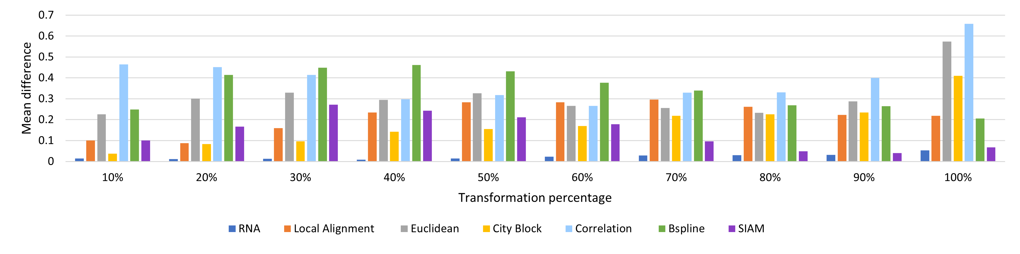
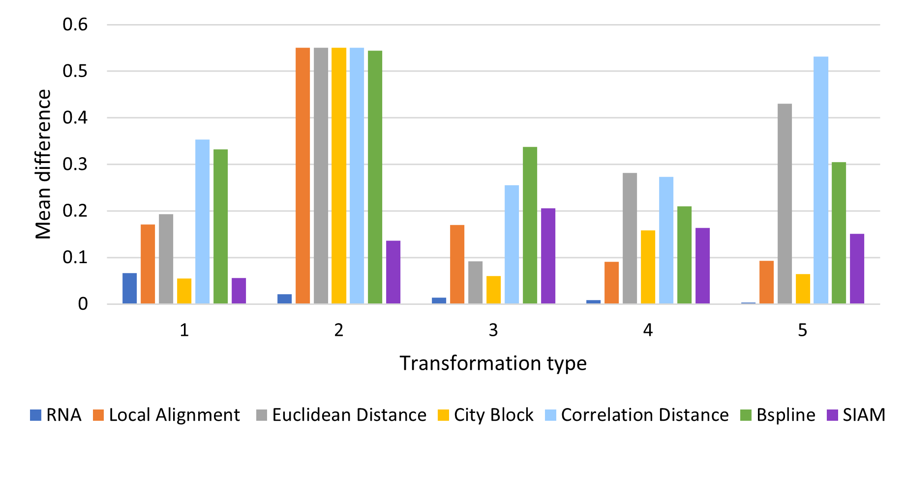
In these experiments a melody is modified with 4 types of modifications and by percentages (10, 20, …, 100). The expected value from each similarity measure after normalization should be equal to the percentage of the modification, for example a melody modified by 10% should have a distance of 0.1 with the original, and of 1.0 for a 100% modification.
The tested modifications made on the melody are:
- Pitch: A pitch in a random position is replaced for a random pitch in the MIDI range.
- Duration: The ticks value for a pitch in a random position is modified with a random value in the range (1 y 4096), the range for a measure in 4/4.
- Pitch and Duration: A pitch in a random position has both pitch and tick value modified by random values described previously.
- Elimination: Random notes are removed from the melody.
- Insertion: Random notes are inserted to the melody.
The experiments were conducted using implementations based from Janssen and Urbano in the case of BSpline.
The corresponding Jupyter notebooks can be found in this respository following this link.
Results
Average Difference by percentage:
Average Difference by Modification Type:
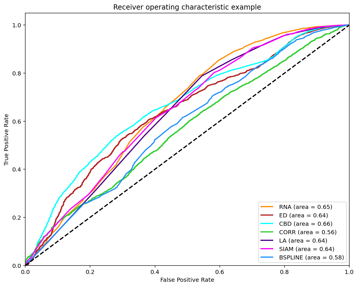
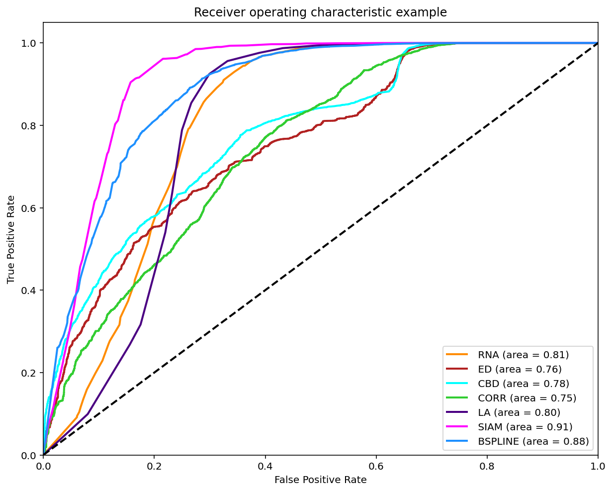
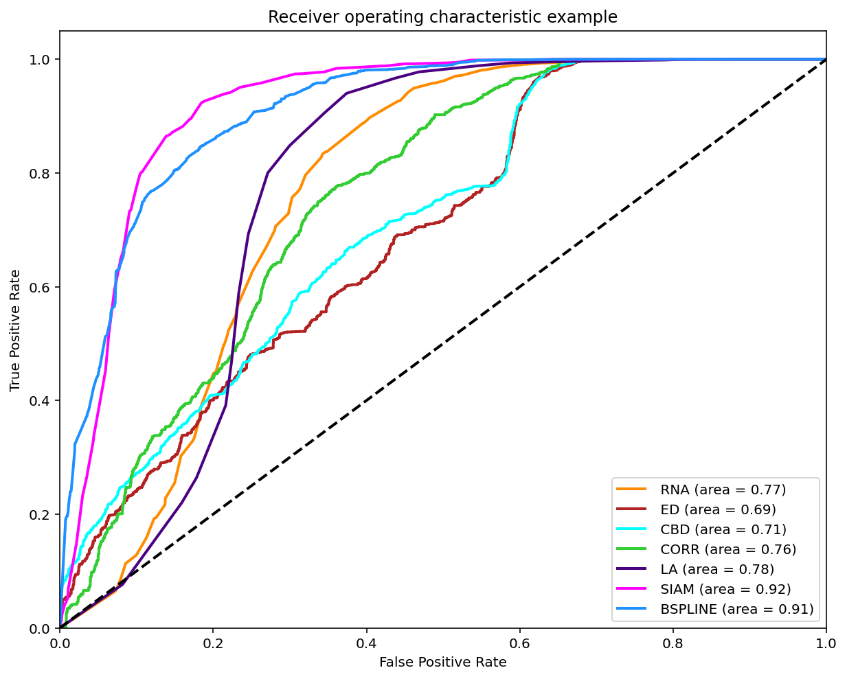
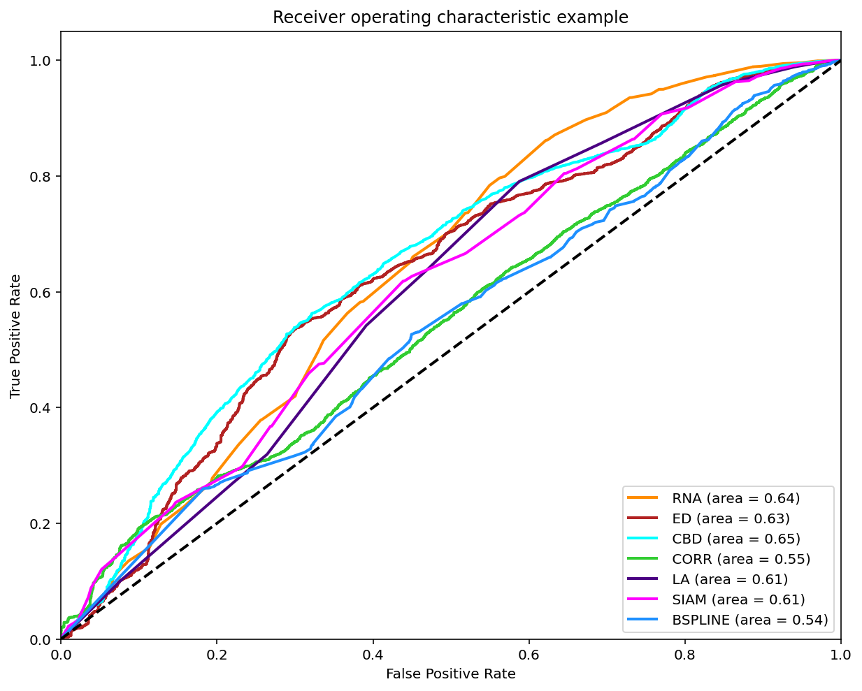
Comparison with Expert annotations
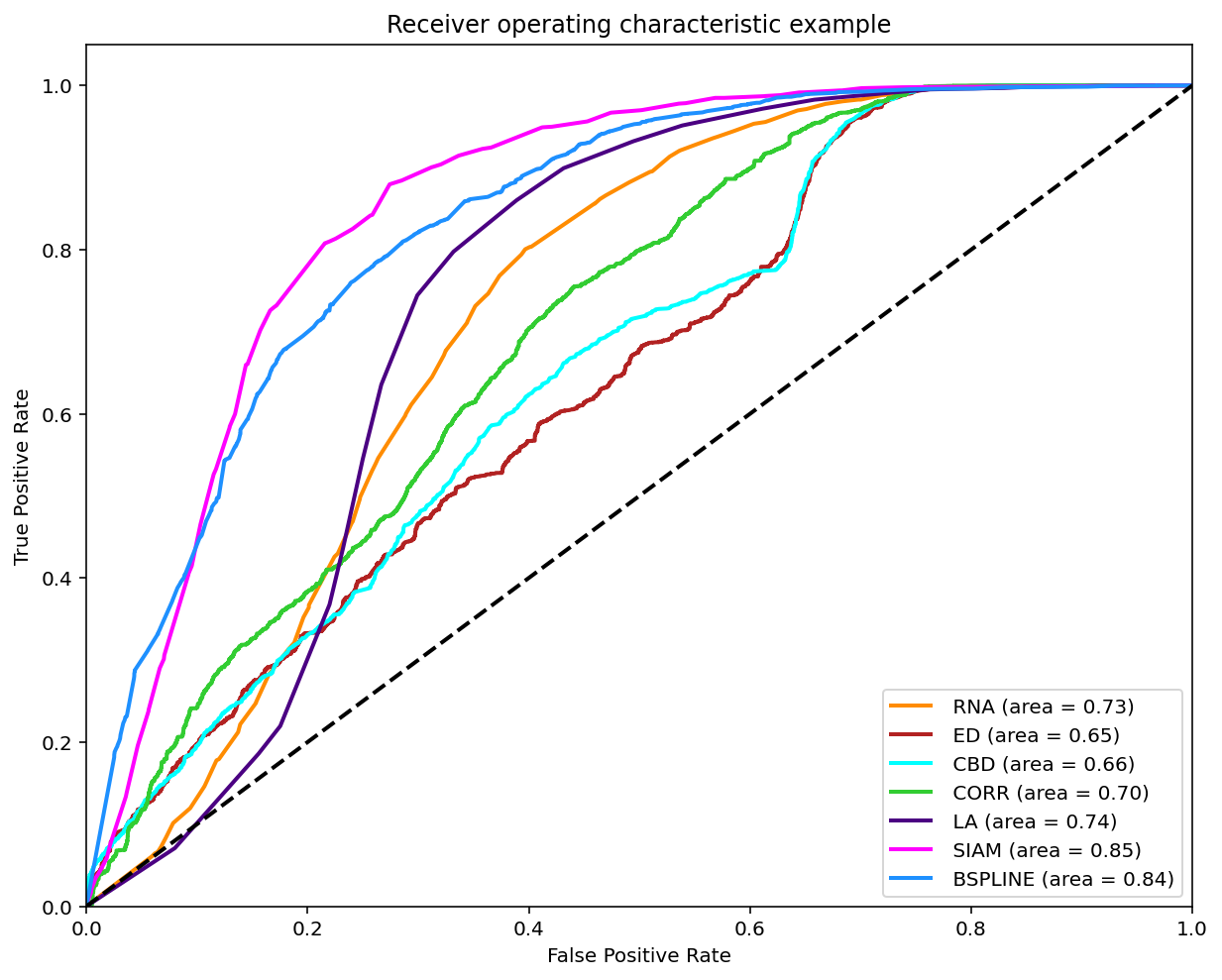
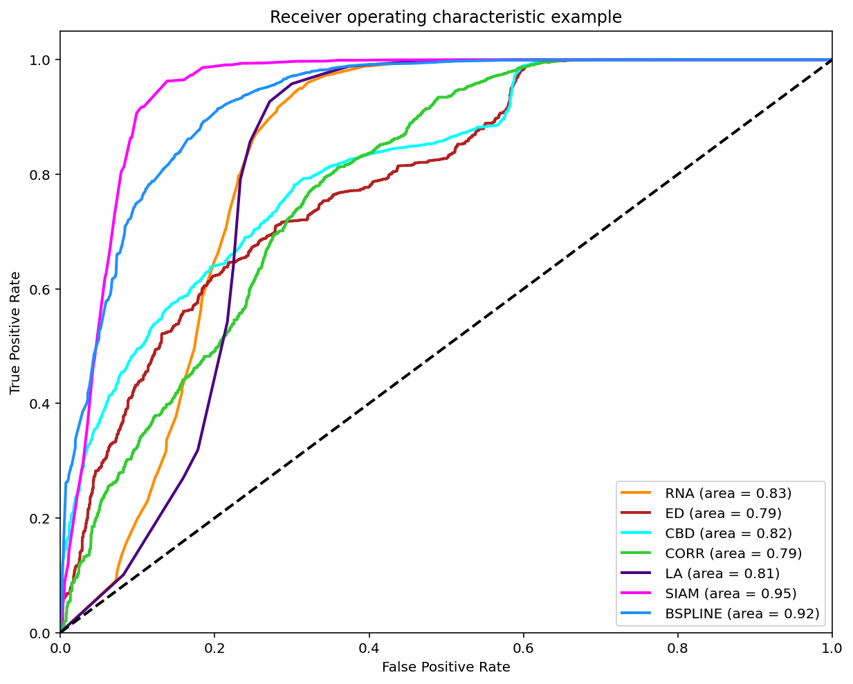
As reviewed in Janssen, et. al. (2017) a classification can be made on the matches found when comparing two melodies in order to compare it with the experts annotations by varying the threshold and ploting the ROC curve.
A modified version of this experiment was made, the main difference is using the similarity measures on all the possible comparissons annotated, that is compare each phrase of each tune to each other per tune family using all 7 similarity measures. The annotations are converted to 0 (identical), 0.5 (somewhat similar) and 1.0 (distinct). To make binary classifications we filtered and splited the data for 3 disctinct experiments. Each experiment took a pair to make the classification. The 3 possible pairs are: 0-0.5, 0.5-1 and 0-1. The reported graph is by taking the majority annotation, if no annotation has the majority the segment is not considered. And for further analysis the same experiments were replicated with filtered segments with an unanimity votes.
The corresponding Jupyter notebooks can be found in this respository following this link. The notebook with the results can be found here.
Results using Majority Vote
Classification (0-0.5)
Classification (0.5-1)
Classification (0-1)
Results using Unanimity Vote
Classification (0-0.5)
Classification (0.5-1)
Classification (0-1)
Summary of F1 Scores
Majority Vote
| Name | 0 - 0.5 | 0.5 - 1 | 0 - 1 |
|---|---|---|---|
| RNA_f1 | 0.7205 | 0.9309 | 0.9521 |
| RNA_precision | 0.5917 | 0.8765 | 0.9206 |
| RNA_recall | 0.9209 | 0.9926 | 0.9859 |
| RNA_specificity | 0.4633 | 0.1053 | 0.5406 |
| ED_f1 | 0.6915 | 0.9281 | 0.9372 |
| ED_precision | 0.5339 | 0.8676 | 0.8863 |
| ED_recall | 0.9812 | 0.9976 | 0.9943 |
| ED_specificity | 0.2765 | 0.0263 | 0.3106 |
| CBD_f1 | 0.6923 | 0.9288 | 0.9383 |
| CBD_precision | 0.5349 | 0.8686 | 0.8868 |
| CBD_recall | 0.9810 | 0.9979 | 0.9960 |
| CBD_specificity | 0.2795 | 0.0344 | 0.3132 |
| CORR_f1 | 0.6984 | 0.9275 | 0.9355 |
| CORR_precision | 0.5510 | 0.8659 | 0.8829 |
| CORR_recall | 0.9536 | 0.9986 | 0.9947 |
| CORR_specificity | 0.3435 | 0.0109 | 0.2874 |
| LA_f1 | 0.7462 | 0.9292 | 0.9552 |
| LA_precision | 0.6377 | 0.8702 | 0.9252 |
| LA_recall | 0.8992 | 0.9967 | 0.9873 |
| LA_specificity | 0.5685 | 0.0487 | 0.5685 |
| SIAM_f1 | 0.7981 | 0.9299 | 0.9677 |
| SIAM_precision | 0.7304 | 0.8742 | 0.9510 |
| SIAM_recall | 0.8796 | 0.9932 | 0.9851 |
| SIAM_specificity | 0.7258 | 0.0855 | 0.7258 |
| BSPLINE_f1 | 0.7588 | 0.9277 | 0.9512 |
| BSPLINE_precision | 0.6795 | 0.8655 | 0.9200 |
| BSPLINE_recall | 0.8590 | 0.9997 | 0.9846 |
| BSPLINE_specificity | 0.6577 | 0.0060 | 0.5375 |
Unanimity Vote
| Name | 0 - 0.5 | 0.5 - 1 | 0 - 1 |
|---|---|---|---|
| RNA_f1 | 0.7048 | 0.9612 | 0.9689 |
| RNA_precision | 0.5605 | 0.9262 | 0.9498 |
| RNA_recall | 0.9493 | 0.9989 | 0.9887 |
| RNA_specificity | 0.5379 | 0.0297 | 0.6051 |
| ED_f1 | 0.6509 | 0.9606 | 0.9581 |
| ED_precision | 0.4901 | 0.9242 | 0.9219 |
| ED_recall | 0.9686 | 1.0000 | 0.9973 |
| ED_specificity | 0.3745 | 0.0012 | 0.3613 |
| CBD_f1 | 0.6519 | 0.9608 | 0.9590 |
| CBD_precision | 0.4889 | 0.9252 | 0.9228 |
| CBD_recall | 0.9779 | 0.9992 | 0.9983 |
| CBD_specificity | 0.3653 | 0.0163 | 0.3680 |
| CORR_f1 | 0.6707 | 0.9606 | 0.9583 |
| CORR_precision | 0.5337 | 0.9241 | 0.9207 |
| CORR_recall | 0.9024 | 1.0000 | 0.9991 |
| CORR_specificity | 0.5105 | 0.0000 | 0.3490 |
| LA_f1 | 0.7394 | 0.9607 | 0.9701 |
| LA_precision | 0.6094 | 0.9243 | 0.9523 |
| LA_recall | 0.9401 | 1.0000 | 0.9885 |
| LA_specificity | 0.6260 | 0.0028 | 0.6260 |
| SIAM_f1 | 0.8315 | 0.9608 | 0.9815 |
| SIAM_precision | 0.7566 | 0.9249 | 0.9697 |
| SIAM_recall | 0.9229 | 0.9995 | 0.9936 |
| SIAM_specificity | 0.8157 | 0.0118 | 0.7651 |
| BSPLINE_f1 | 0.7903 | 0.9606 | 0.9704 |
| BSPLINE_precision | 0.7410 | 0.9241 | 0.9527 |
| BSPLINE_recall | 0.8465 | 1.0000 | 0.9887 |
| BSPLINE_specificity | 0.8163 | 0.0000 | 0.6292 |
Summary of Best ROC Values (closest to tpr=1.0 and fpr=0.0)
Majority Vote
| Name | 0 - 0.5 | 0.5 - 1 | 0 - 1 |
|---|---|---|---|
| RNA_best_roc_value | 0.4037 | 0.2571 | 0.5856 |
| RNA_best_roc_f1 | 0.7052 | 0.8778 | 0.9328 |
| RNA_best_roc_precision | 0.6302 | 0.9014 | 0.9359 |
| RNA_best_roc_recall | 0.8005 | 0.8553 | 0.9298 |
| RNA_best_roc_specificity | 0.6032 | 0.4017 | 0.6557 |
| ED_best_roc_value | 0.2656 | 0.2278 | 0.3704 |
| ED_best_roc_f1 | 0.6897 | 0.6718 | 0.7569 |
| ED_best_roc_precision | 0.5390 | 0.9182 | 0.9278 |
| ED_best_roc_recall | 0.9574 | 0.5297 | 0.6392 |
| ED_best_roc_specificity | 0.3082 | 0.6981 | 0.7312 |
| CBD_best_roc_value | 0.2681 | 0.2565 | 0.4215 |
| CBD_best_roc_f1 | 0.6900 | 0.6801 | 0.8490 |
| CBD_best_roc_precision | 0.5401 | 0.9244 | 0.9208 |
| CBD_best_roc_recall | 0.9549 | 0.5380 | 0.7877 |
| CBD_best_roc_specificity | 0.3132 | 0.7186 | 0.6338 |
| CORR_best_roc_value | 0.3141 | 0.0955 | 0.3737 |
| CORR_best_roc_f1 | 0.6630 | 0.7153 | 0.8577 |
| CORR_best_roc_precision | 0.5915 | 0.8838 | 0.9092 |
| CORR_best_roc_recall | 0.7540 | 0.6007 | 0.8117 |
| CORR_best_roc_specificity | 0.5601 | 0.4948 | 0.5620 |
| LA_best_roc_value | 0.4712 | 0.2435 | 0.6254 |
| LA_best_roc_f1 | 0.7413 | 0.8417 | 0.9340 |
| LA_best_roc_precision | 0.6513 | 0.9025 | 0.9435 |
| LA_best_roc_recall | 0.8602 | 0.7886 | 0.9247 |
| LA_best_roc_specificity | 0.6111 | 0.4549 | 0.7008 |
| SIAM_best_roc_value | 0.6054 | 0.2198 | 0.7474 |
| SIAM_best_roc_f1 | 0.7981 | 0.8480 | 0.9397 |
| SIAM_best_roc_precision | 0.7304 | 0.8980 | 0.9674 |
| SIAM_best_roc_recall | 0.8796 | 0.8032 | 0.9136 |
| SIAM_best_roc_specificity | 0.7258 | 0.4166 | 0.8339 |
| BSPLINE_best_roc_value | 0.5238 | 0.1299 | 0.6274 |
| BSPLINE_best_roc_f1 | 0.7539 | 0.7282 | 0.9291 |
| BSPLINE_best_roc_precision | 0.7051 | 0.8902 | 0.9452 |
| BSPLINE_best_roc_recall | 0.8099 | 0.6161 | 0.9136 |
| BSPLINE_best_roc_specificity | 0.7139 | 0.5138 | 0.7139 |
Unanimity Vote
| Name | 0 - 0.5 | 0.5 - 1 | 0 - 1 |
|---|---|---|---|
| RNA_best_roc_value | 0.4932 | 0.2401 | 0.6398 |
| RNA_best_roc_f1 | 0.7042 | 0.9010 | 0.9542 |
| RNA_best_roc_precision | 0.5797 | 0.9441 | 0.9586 |
| RNA_best_roc_recall | 0.8968 | 0.8616 | 0.9498 |
| RNA_best_roc_specificity | 0.5963 | 0.3785 | 0.6901 |
| ED_best_roc_value | 0.3432 | 0.2364 | 0.4305 |
| ED_best_roc_f1 | 0.6509 | 0.6859 | 0.8123 |
| ED_best_roc_precision | 0.4902 | 0.9562 | 0.9506 |
| ED_best_roc_recall | 0.9684 | 0.5347 | 0.7092 |
| ED_best_roc_specificity | 0.3748 | 0.7017 | 0.7214 |
| CBD_best_roc_value | 0.3432 | 0.2409 | 0.4788 |
| CBD_best_roc_f1 | 0.6519 | 0.7080 | 0.8582 |
| CBD_best_roc_precision | 0.4889 | 0.9552 | 0.9512 |
| CBD_best_roc_recall | 0.9779 | 0.5625 | 0.7818 |
| CBD_best_roc_specificity | 0.3653 | 0.6784 | 0.6970 |
| CORR_best_roc_value | 0.4157 | 0.0918 | 0.4522 |
| CORR_best_roc_f1 | 0.6586 | 0.3240 | 0.8638 |
| CORR_best_roc_precision | 0.5721 | 0.9584 | 0.9461 |
| CORR_best_roc_recall | 0.7758 | 0.1950 | 0.7947 |
| CORR_best_roc_specificity | 0.6399 | 0.8968 | 0.6575 |
| LA_best_roc_value | 0.5660 | 0.2031 | 0.6579 |
| LA_best_roc_f1 | 0.7394 | 0.8600 | 0.9590 |
| LA_best_roc_precision | 0.6094 | 0.9425 | 0.9602 |
| LA_best_roc_recall | 0.9401 | 0.7907 | 0.9578 |
| LA_best_roc_specificity | 0.6260 | 0.4124 | 0.7001 |
| SIAM_best_roc_value | 0.7386 | 0.1799 | 0.8243 |
| SIAM_best_roc_f1 | 0.8315 | 0.7476 | 0.9720 |
| SIAM_best_roc_precision | 0.7566 | 0.9450 | 0.9813 |
| SIAM_best_roc_recall | 0.9229 | 0.6184 | 0.9629 |
| SIAM_best_roc_specificity | 0.8157 | 0.5615 | 0.8614 |
| BSPLINE_best_roc_value | 0.6629 | 0.0774 | 0.7106 |
| BSPLINE_best_roc_f1 | 0.7903 | 0.4070 | 0.9422 |
| BSPLINE_best_roc_precision | 0.7410 | 0.9455 | 0.9713 |
| BSPLINE_best_roc_recall | 0.8465 | 0.2593 | 0.9147 |
| BSPLINE_best_roc_specificity | 0.8163 | 0.8181 | 0.7959 |
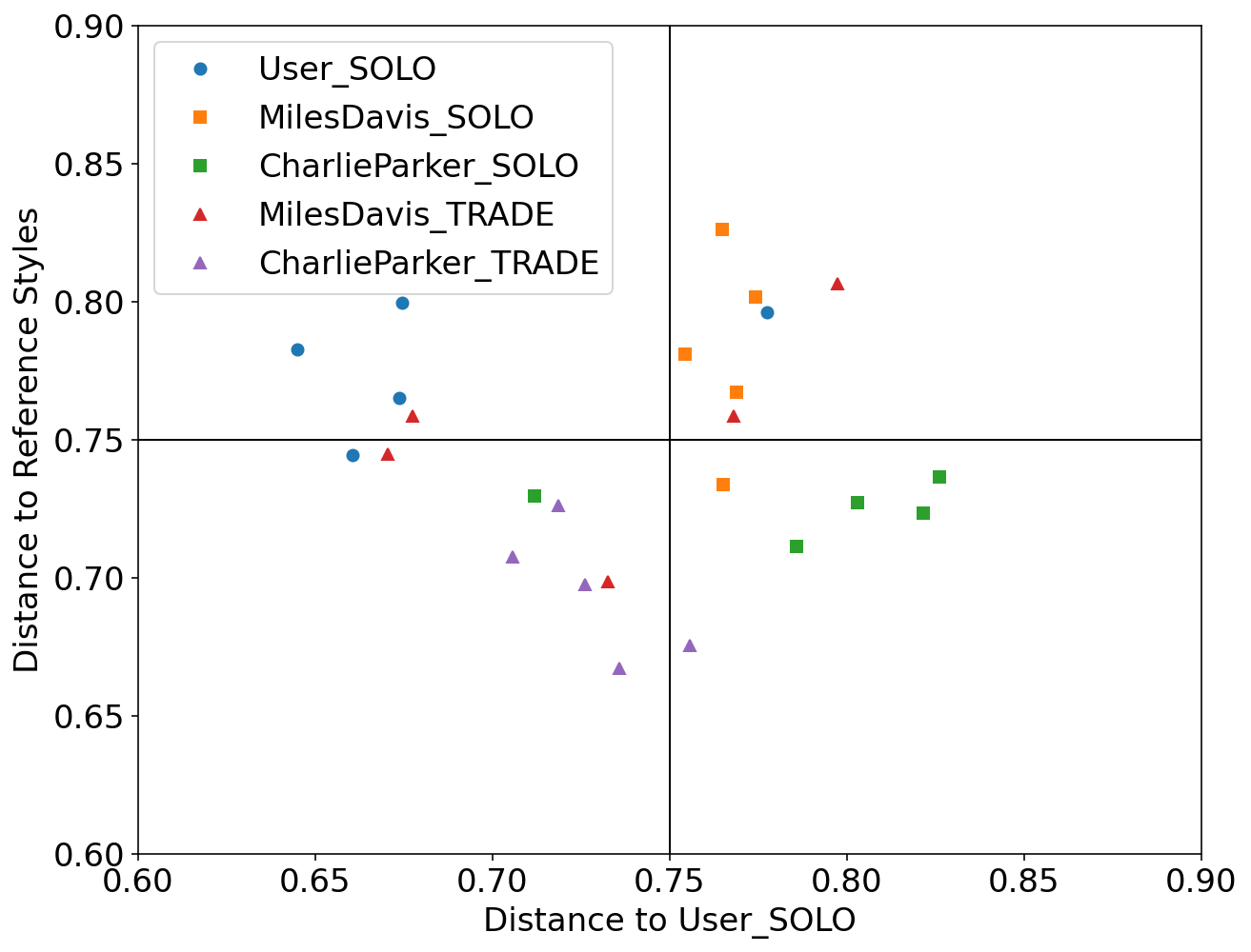
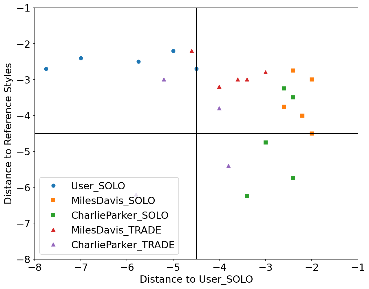
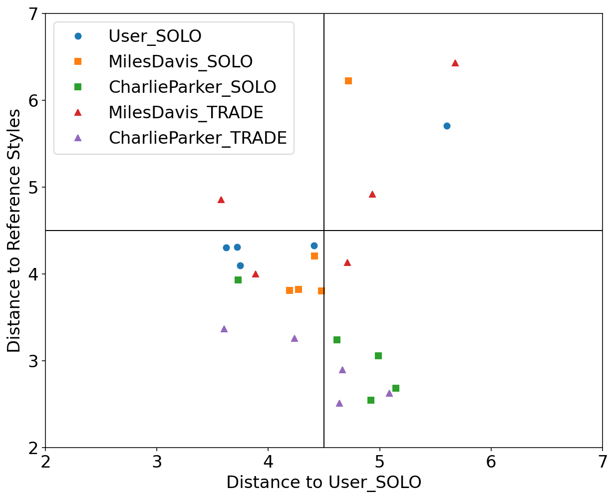
Case study using Impro-Visor
We used Impro-Visor to test the similarity measures that had the best results in our controlled experiments and for comparison is included a simple measure that is Euclidean Distance. For each group of melodies the similarity was calculated for the X axis to the Corpus created by the user. For the Y axis it was calculated with the corresponding solos of the composer pre-built grammar. For example the Tradings between User and Miles Davis were compared with User’s corpus for the X axis and with the grammar solos of Miles Davis for the Y axis.
The following melodies were used:
Corpus - User
Original pieces composed by an User, they are 12 measures in length.
Grammar Solo - Miles Davis
Using the pre-built grammar for Miles Davis in Impro-Visor, 5 melodies of similar length of 12 measures were generated.
Grammar Solo - Charlie Parker
Using the pre-built grammar for Charlie Parker in Impro-Visor, 5 melodies of similar length of 12 measures were generated.
Trading - User & Charlie Parker
With an active trade using 2 measures for each turn for a total of 12 measures, the User was asked to improvise using the prebuilt grammar of Charlie Parker.
Trading - User & Miles Davis
With an active trade using 2 measures for each turn for a total of 12 measures, the user was asked to improvise using the prebuilt grammar of Miles Davis.
Results
RNA:
 SIAM:
SIAM:
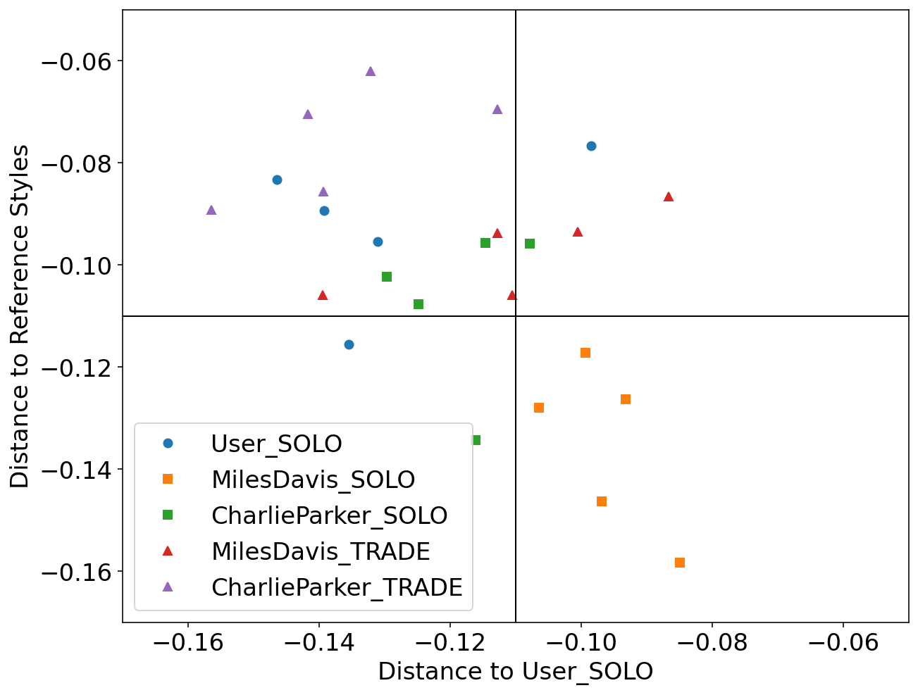 Local Alignment:
 Euclidean Distance:
The corresponding Jupyter notebooks can be found in this respository following this link.